Microbiome Project
Jie Zhou
11/9/2021
Last updated: 2022-04-12
Checks: 5 2
Knit directory: Cystic-Fibrosis-and-Gut-Microbiome/
This reproducible R Markdown analysis was created with workflowr (version 1.7.0). The Checks tab describes the reproducibility checks that were applied when the results were created. The Past versions tab lists the development history.
The R Markdown is untracked by Git. To know which version of the R Markdown file created these results, you’ll want to first commit it to the Git repo. If you’re still working on the analysis, you can ignore this warning. When you’re finished, you can run wflow_publish to commit the R Markdown file and build the HTML.
Great job! The global environment was empty. Objects defined in the global environment can affect the analysis in your R Markdown file in unknown ways. For reproduciblity it’s best to always run the code in an empty environment.
The command set.seed(20181210) was run prior to running the code in the R Markdown file. Setting a seed ensures that any results that rely on randomness, e.g. subsampling or permutations, are reproducible.
Great job! Recording the operating system, R version, and package versions is critical for reproducibility.
Nice! There were no cached chunks for this analysis, so you can be confident that you successfully produced the results during this run.
Using absolute paths to the files within your workflowr project makes it difficult for you and others to run your code on a different machine. Change the absolute path(s) below to the suggested relative path(s) to make your code more reproducible.
| absolute | relative |
|---|---|
| C:/Users/Jie Zhou/Documents/paper02052022/longitudinalOutcome/Cystic-Fibrosis-and-Gut-Microbiome/data/ddata.csv | data/ddata.csv |
| C:/Users/Jie Zhou/Documents/paper02052022/longitudinalOutcome/Cystic-Fibrosis-and-Gut-Microbiome/data/analyst_pulmonary_exacerbation_202110061618.csv | data/analyst_pulmonary_exacerbation_202110061618.csv |
Great! You are using Git for version control. Tracking code development and connecting the code version to the results is critical for reproducibility.
The results in this page were generated with repository version f041e9d. See the Past versions tab to see a history of the changes made to the R Markdown and HTML files.
Note that you need to be careful to ensure that all relevant files for the analysis have been committed to Git prior to generating the results (you can use wflow_publish or wflow_git_commit). workflowr only checks the R Markdown file, but you know if there are other scripts or data files that it depends on. Below is the status of the Git repository when the results were generated:
Ignored files:
    Ignored:    .RData
    Ignored:    .Rhistory
    Ignored:    .Rproj.user/

Untracked files:
    Untracked:  analysis/Poission regression model.Rmd
    Untracked:  analysis/Poission-regression-model.Rmd

Unstaged changes:
    Modified:   analysis/index.Rmd
    Modified:   analysis/marginal model.Rmd
    Modified:   analysis/pca of relative abundance of microbiome.Rmd
    Modified:   analysis/random effect model.Rmd
    Modified:   analysis/survival model.Rmd
Note that any generated files, e.g. HTML, png, CSS, etc., are not included in this status report because it is ok for generated content to have uncommitted changes.
There are no past versions. Publish this analysis with wflow_publish() to start tracking its development.
Input the microbiome data: 38 subjects, 82 microbes. These data have undergone log-ratio transfomation and so can be deemed as normal data. As for the Outcome data also is input in a separate file.
taxa_raw = read.csv("C:/Users/Jie Zhou/Documents/paper02052022/longitudinalOutcome/Cystic-Fibrosis-and-Gut-Microbiome/data/ddata.csv")
# averaging across time points
taxa_avg = taxa_raw %>%
  group_by(subject) %>%
  summarize_all(list(mean))

taxa = taxa_avg[,4:ncol(taxa_avg)]
pulm = read.delim("C:/Users/Jie Zhou/Documents/paper02052022/longitudinalOutcome/Cystic-Fibrosis-and-Gut-Microbiome/data/analyst_pulmonary_exacerbation_202110061618.csv")
Selecting the microbial interaction network using glasso. Here the tuning parameter is recommended based on previous study. Given the selected network, leadeigen algorithm is employed to find the communities in the network.
set.seed(2)
# lambda_glasso = seq(0.05, 6, 0.01)
# cv_glasso_taxa = CVglasso(taxa, K = 5, lam = lambda_glasso)
#   lam_pick = cv_glasso_taxa$Tuning[2]
lam_pick=0.75
glasso_taxa = glasso(cov(taxa), rho = lam_pick)
pcov_taxa = glasso_taxa$wi
taxa_nwk = as.matrix(ifelse(pcov_taxa != 0, 1, 0))
# graph theory

taxa_graph = graph.adjacency(taxa_nwk, mode = "undirected")
taxa_louvain = cluster_louvain(taxa_graph)
taxa_leadeigen = cluster_leading_eigen(taxa_graph) # This one produces fewer modules (clusters)
For each of the communities, compute its principal components.
colnames(taxa[which(taxa_leadeigen$membership == 3)]) [1] "Erysipelatoclostridium" "Bacteroides" "Parabacteroides"
[4] "Tyzzerella" "Mediterraneibacter" "Sellimonas"
[7] "Flavonifractor" "Ruminococcus2" "Ruthenibacterium"
[10] "Alistipes" "Clostridium_XVIII" "Monoglobus"
[13] "Eggerthella" "Turicibacter" "Eisenbergiella"
[16] "Flintibacter" "Agathobaculum" "Anaerotignum"
[19] "Dysosmobacter" "Bilophila" "Clostridium_IV"
[22] "Faecalicatena" taxa_le_cluster1 = taxa[which(taxa_leadeigen$membership == 1)]
taxa_le_pca1 = prcomp(taxa_le_cluster1)
taxa_le_eigen1 = as.matrix(taxa_le_cluster1) %*% taxa_le_pca1$rotation
plot(taxa_le_pca1$sdev^2/sum(taxa_le_pca1$sdev^2), type="l", main = "Leading Eigen Cluster 1 PCs",
xlab="principle components", ylab="variance explained")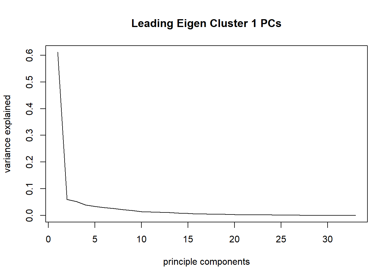
fig.path you set was ignored by workflowr.
plot(taxa_le_eigen1[,1], taxa_le_eigen1[,2], main = "First cluster",
     xlab="PCA1", ylab="PCA2")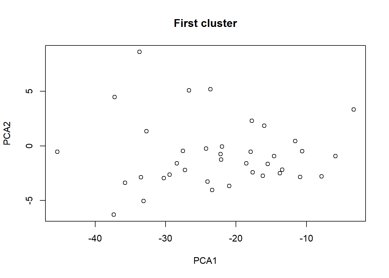
fig.path you set was ignored by workflowr.
summary(taxa_le_pca1)Importance of components:
PC1 PC2 PC3 PC4 PC5 PC6 PC7
Standard deviation 9.7474 3.04649 2.85256 2.46476 2.28825 2.14601 2.02753
Proportion of Variance 0.6113 0.05971 0.05235 0.03908 0.03369 0.02963 0.02645
Cumulative Proportion 0.6113 0.67099 0.72334 0.76242 0.79611 0.82574 0.85219
PC8 PC9 PC10 PC11 PC12 PC13 PC14
Standard deviation 1.83713 1.69675 1.49252 1.43282 1.39194 1.30321 1.20289
Proportion of Variance 0.02171 0.01852 0.01433 0.01321 0.01247 0.01093 0.00931
Cumulative Proportion 0.87390 0.89242 0.90675 0.91996 0.93243 0.94335 0.95266
PC15 PC16 PC17 PC18 PC19 PC20 PC21
Standard deviation 1.08809 0.95990 0.91115 0.87864 0.79410 0.75140 0.66717
Proportion of Variance 0.00762 0.00593 0.00534 0.00497 0.00406 0.00363 0.00286
Cumulative Proportion 0.96028 0.96621 0.97155 0.97652 0.98057 0.98421 0.98707
PC22 PC23 PC24 PC25 PC26 PC27 PC28
Standard deviation 0.63713 0.59364 0.55947 0.53479 0.44205 0.39067 0.30968
Proportion of Variance 0.00261 0.00227 0.00201 0.00184 0.00126 0.00098 0.00062
Cumulative Proportion 0.98968 0.99195 0.99396 0.99580 0.99706 0.99804 0.99866
PC29 PC30 PC31 PC32 PC33
Standard deviation 0.29779 0.23523 0.19061 0.15304 0.06929
Proportion of Variance 0.00057 0.00036 0.00023 0.00015 0.00003
Cumulative Proportion 0.99923 0.99958 0.99982 0.99997 1.00000taxa_le_cluster2 = taxa[which(taxa_leadeigen$membership == 2)]
taxa_le_pca2 = prcomp(taxa_le_cluster2)
taxa_le_eigen2 = as.matrix(taxa_le_cluster2) %*% taxa_le_pca2$rotation
plot(taxa_le_pca2$sdev^2/sum(taxa_le_pca2$sdev^2), type="l", main = "Leading Eigen Cluster 2 PCs",
xlab="principle components", ylab="variance explained")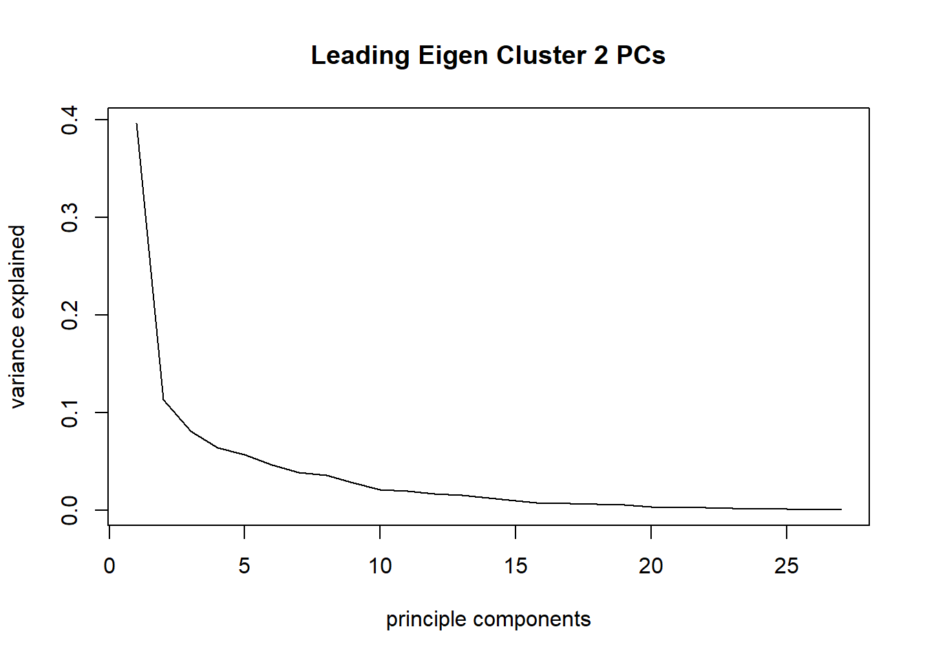
fig.path you set was ignored by workflowr.
plot(taxa_le_eigen2[,1], taxa_le_eigen2[,2], main = "Second cluster",
     xlab="PCA1", ylab="PCA2")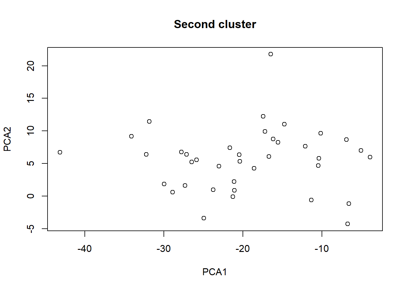
fig.path you set was ignored by workflowr.
summary(taxa_le_pca2)Importance of components:
PC1 PC2 PC3 PC4 PC5 PC6 PC7
Standard deviation 9.0411 4.8374 4.08913 3.63476 3.44137 3.09360 2.82121
Proportion of Variance 0.3961 0.1134 0.08102 0.06401 0.05738 0.04637 0.03857
Cumulative Proportion 0.3961 0.5094 0.59047 0.65448 0.71187 0.75824 0.79680
PC8 PC9 PC10 PC11 PC12 PC13 PC14
Standard deviation 2.71755 2.40777 2.07910 2.03113 1.85601 1.77656 1.63739
Proportion of Variance 0.03578 0.02809 0.02094 0.01999 0.01669 0.01529 0.01299
Cumulative Proportion 0.83259 0.86068 0.88162 0.90161 0.91830 0.93360 0.94659
PC15 PC16 PC17 PC18 PC19 PC20 PC21
Standard deviation 1.44161 1.24244 1.22847 1.15619 1.08041 0.89318 0.80377
Proportion of Variance 0.01007 0.00748 0.00731 0.00648 0.00566 0.00387 0.00313
Cumulative Proportion 0.95666 0.96414 0.97145 0.97793 0.98358 0.98745 0.99058
PC22 PC23 PC24 PC25 PC26 PC27
Standard deviation 0.74307 0.6581 0.60150 0.51462 0.44220 0.37021
Proportion of Variance 0.00268 0.0021 0.00175 0.00128 0.00095 0.00066
Cumulative Proportion 0.99325 0.9953 0.99711 0.99839 0.99934 1.00000taxa_le_cluster3= taxa[which(taxa_leadeigen$membership == 3)]
taxa_le_pca3 = prcomp(taxa_le_cluster3)
taxa_le_eigen3 = as.matrix(taxa_le_cluster3) %*% taxa_le_pca3$rotation
plot(taxa_le_pca3$sdev^2/sum(taxa_le_pca3$sdev^2), type="l", main = "Leading Eigen Cluster 3 PCs",
xlab="principle components", ylab="variance explained")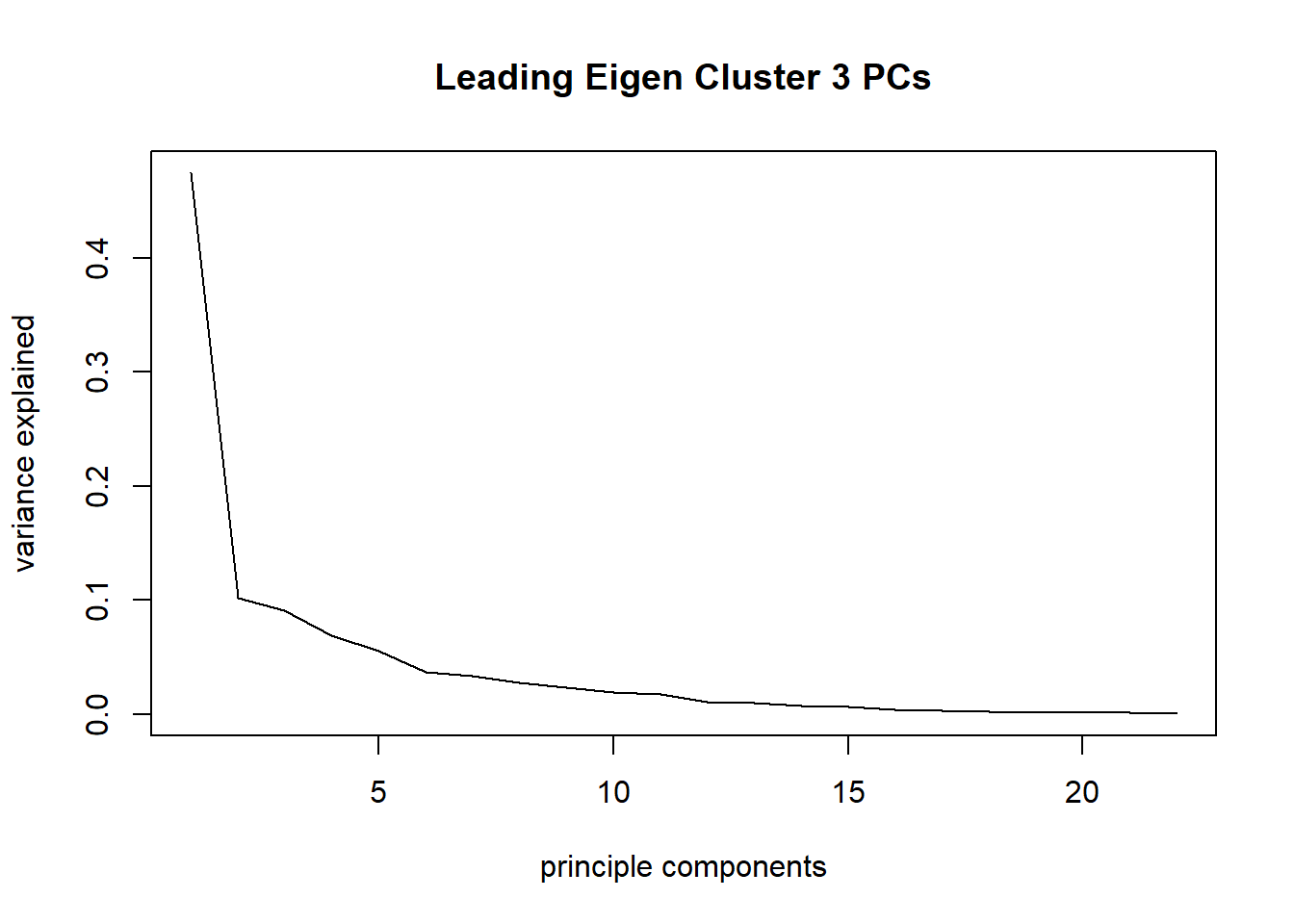
fig.path you set was ignored by workflowr.
plot(taxa_le_eigen3[,1], taxa_le_eigen3[,2], main = "Third cluster",
     xlab="PCA1", ylab="PCA2")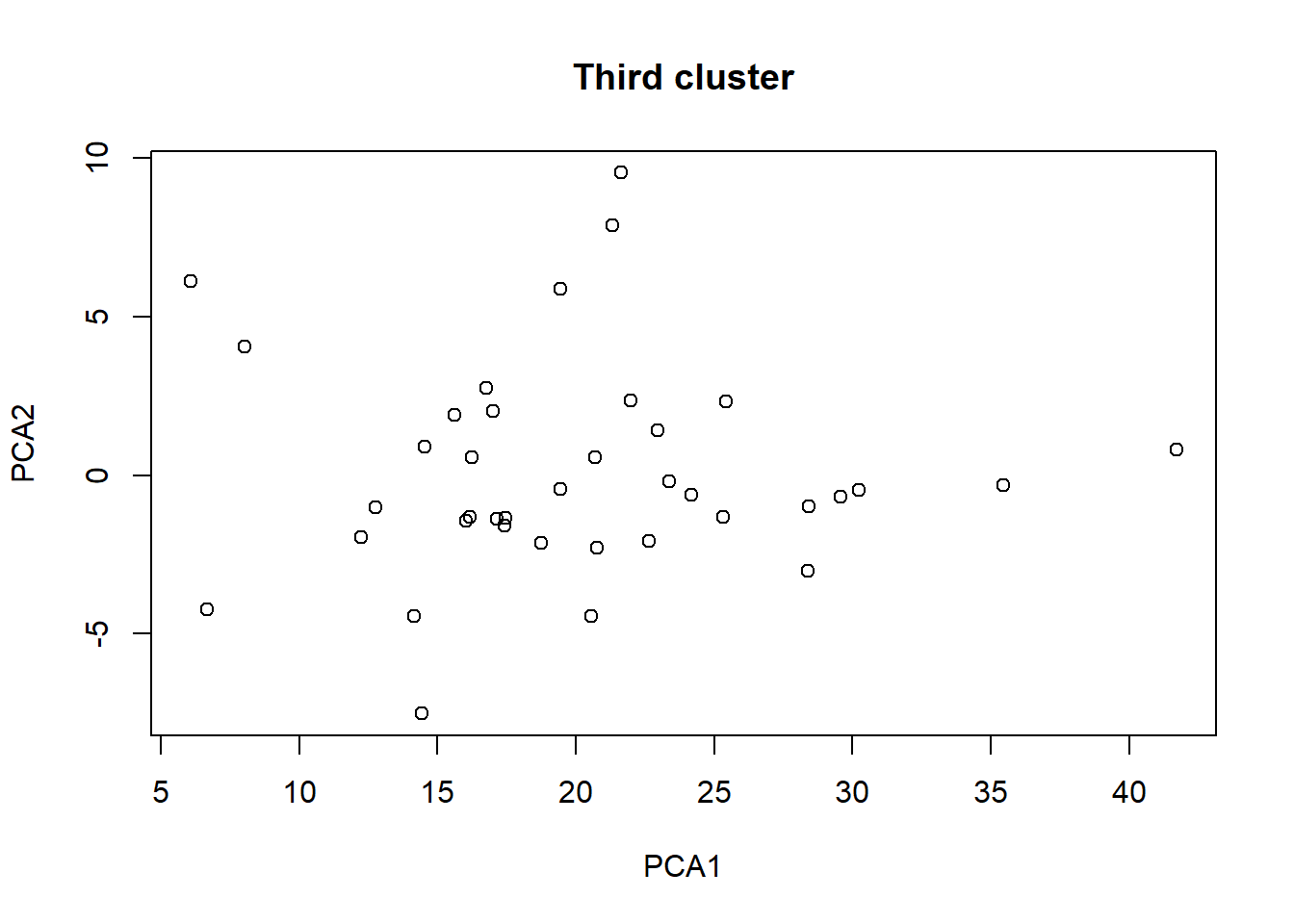
fig.path you set was ignored by workflowr.
summary(taxa_le_pca3)Importance of components:
PC1 PC2 PC3 PC4 PC5 PC6 PC7
Standard deviation 7.3329 3.3965 3.20515 2.8028 2.5060 2.04305 1.94407
Proportion of Variance 0.4743 0.1018 0.09062 0.0693 0.0554 0.03682 0.03334
Cumulative Proportion 0.4743 0.5761 0.66674 0.7360 0.7914 0.82826 0.86160
PC8 PC9 PC10 PC11 PC12 PC13 PC14
Standard deviation 1.76180 1.64773 1.49647 1.41514 1.11306 1.0542 0.92463
Proportion of Variance 0.02738 0.02395 0.01976 0.01767 0.01093 0.0098 0.00754
Cumulative Proportion 0.88898 0.91294 0.93269 0.95036 0.96129 0.9711 0.97863
PC15 PC16 PC17 PC18 PC19 PC20 PC21
Standard deviation 0.88317 0.68642 0.59050 0.50156 0.44078 0.39739 0.3842
Proportion of Variance 0.00688 0.00416 0.00308 0.00222 0.00171 0.00139 0.0013
Cumulative Proportion 0.98551 0.98967 0.99274 0.99496 0.99668 0.99807 0.9994
PC22
Standard deviation 0.26658
Proportion of Variance 0.00063
Cumulative Proportion 1.00000Linking Outcome
These are the pulmonary exacerbation events that have been entered into the database. As you will notice, there are often multiple events per person.
Not all patients or patient IDs on this list have a 16S microbiome sequence.
Note that pe_occurence=1 - is a definite yes; 2 is no (but was previously entered as having a PE due to some mild PE symptoms) and 3 is unknown. As a sensitivity analysis, you can exclude 2 and 3 to see if your deductions change.
If pe_occurence is missing, you can exclude unless the comments indicate otherwise.
Dates are sometimes missing when the pe_date was unknown; use event_date instead,
taxa_short = taxa_avg %>%
  filter(subject %in% unique(pulm$patient_id))
pulm_new = pulm %>% group_by(patient_id) %>%
  filter(patient_id %in% (taxa_avg$subject[taxa_avg$subject %in% unique(pulm$patient_id)]))
pulm_new$pe_occurance = ifelse(pulm_new$pe_occurance <=1, 1, 0)
pulm_new = pulm_new %>%
  summarise(pulmonary = sum(pe_occurance, na.rm = T))
colnames(pulm_new) = c("subject", "pe")

taxa_merge = left_join(taxa_short, pulm_new, by = "subject")

#View(taxa_merge[c("subject", "pe")])
Poisson regression: first pcs for each of three clusters
# Get eigentaxa
index_final = which(taxa_avg$subject %in% taxa_merge$subject)
## first pc for each cluster
taxa_pois = as.data.frame(cbind(taxa_le_eigen1[index_final,1],
      taxa_le_eigen2[index_final,1],
      taxa_le_eigen3[index_final,1],
      taxa_merge$pe,
      ifelse(taxa_merge$pe == 0, 0, 1)))
colnames(taxa_pois) = c("taxa_eigen1", "taxa_eigen2", "taxa_eigen3",
                        "pe", "pe_bi")
summary(glm(pe ~ taxa_eigen1 + taxa_eigen2 + taxa_eigen3, family = "poisson", control = glm.control(maxit = 50),data = taxa_pois))
Call:
glm(formula = pe ~ taxa_eigen1 + taxa_eigen2 + taxa_eigen3, family = "poisson",
    data = taxa_pois, control = glm.control(maxit = 50))

Deviance Residuals:
    Min       1Q   Median       3Q      Max
-1.5930  -0.6063  -0.2631   0.4297   1.4278

Coefficients:
              Estimate Std. Error z value Pr(>|z|)
(Intercept)  0.7103003  0.9064313   0.784   0.4333
taxa_eigen1  0.0682120  0.0292852   2.329   0.0198 *
taxa_eigen2 -0.0670223  0.0324842  -2.063   0.0391 *
taxa_eigen3  0.0007441  0.0525040   0.014   0.9887
---
Signif. codes:  0 '***' 0.001 '**' 0.01 '*' 0.05 '.' 0.1 ' ' 1

(Dispersion parameter for poisson family taken to be 1)

    Null deviance: 18.995  on 17  degrees of freedom
Residual deviance: 11.391  on 14  degrees of freedom
AIC: 58.988

Number of Fisher Scoring iterations: 5
Poisson regression: first pcs for each of three clusters
# Get eigentaxa
index_final = which(taxa_avg$subject %in% taxa_merge$subject)
## first pc for each cluster
taxa_pois = as.data.frame(cbind(taxa_le_eigen1[index_final,1], taxa_le_eigen1[index_final,2],
      taxa_le_eigen2[index_final,1],
      taxa_le_eigen2[index_final,2],
      taxa_le_eigen3[index_final,1],
      taxa_le_eigen3[index_final,2],
      taxa_merge$pe,
      ifelse(taxa_merge$pe == 0, 0, 1)))
colnames(taxa_pois) = c("taxa_eigen11","taxa_eigen12", "taxa_eigen21","taxa_eigen22", "taxa_eigen31","taxa_eigen32",
                        "pe", "pe_bi")
summary(glm(pe ~ taxa_eigen11 + taxa_eigen12+ taxa_eigen21 +  taxa_eigen22+ taxa_eigen31+ taxa_eigen32, family = "poisson", control = glm.control(maxit = 50),data = taxa_pois))
Call:
glm(formula = pe ~ taxa_eigen11 + taxa_eigen12 + taxa_eigen21 +
    taxa_eigen22 + taxa_eigen31 + taxa_eigen32, family = "poisson",
    data = taxa_pois, control = glm.control(maxit = 50))

Deviance Residuals:
    Min       1Q   Median       3Q      Max
-1.6485  -0.4101  -0.2211   0.3466   1.3566

Coefficients:
             Estimate Std. Error z value Pr(>|z|)
(Intercept)   0.94751    1.38892   0.682   0.4951
taxa_eigen11  0.05834    0.04325   1.349   0.1773
taxa_eigen12 -0.04583    0.13470  -0.340   0.7337
taxa_eigen21 -0.08593    0.04017  -2.139   0.0324 *
taxa_eigen22 -0.02758    0.08126  -0.339   0.7343
taxa_eigen31 -0.03590    0.08427  -0.426   0.6701
taxa_eigen32 -0.15042    0.15247  -0.987   0.3239
---
Signif. codes:  0 '***' 0.001 '**' 0.01 '*' 0.05 '.' 0.1 ' ' 1

(Dispersion parameter for poisson family taken to be 1)

    Null deviance: 18.995  on 17  degrees of freedom
Residual deviance: 10.380  on 11  degrees of freedom
AIC: 63.977

Number of Fisher Scoring iterations: 5
sessionInfo()R version 4.1.2 (2021-11-01)
Platform: x86_64-w64-mingw32/x64 (64-bit)
Running under: Windows 10 x64 (build 19043)
Matrix products: default
locale:
[1] LC_COLLATE=English_United States.1252
[2] LC_CTYPE=English_United States.1252
[3] LC_MONETARY=English_United States.1252
[4] LC_NUMERIC=C
[5] LC_TIME=English_United States.1252
attached base packages:
[1] parallel stats graphics grDevices utils datasets methods
[8] base
other attached packages:
[1] corrplot_0.92 glmnet_4.1-3 Matrix_1.3-4
[4] glasso_1.11 sna_2.6 network_1.17.1
[7] statnet.common_4.5.0 GGally_2.1.2 intergraph_2.0-2
[10] ggplot2_3.3.5 igraph_1.2.11 CVglasso_1.0
[13] doParallel_1.0.17 iterators_1.0.14 foreach_1.5.2
[16] tidyr_1.2.0 magrittr_2.0.2 dplyr_1.0.8
[19] data.table_1.14.2
loaded via a namespace (and not attached):
[1] Rcpp_1.0.8 lattice_0.20-45 rprojroot_2.0.2 digest_0.6.29
[5] utf8_1.2.2 R6_2.5.1 plyr_1.8.6 evaluate_0.14
[9] coda_0.19-4 highr_0.9 pillar_1.7.0 rlang_1.0.1
[13] rstudioapi_0.13 jquerylib_0.1.4 rmarkdown_2.11 splines_4.1.2
[17] stringr_1.4.0 munsell_0.5.0 compiler_4.1.2 httpuv_1.6.5
[21] xfun_0.29 pkgconfig_2.0.3 shape_1.4.6 htmltools_0.5.2
[25] tidyselect_1.1.1 tibble_3.1.6 workflowr_1.7.0 codetools_0.2-18
[29] reshape_0.8.8 fansi_1.0.2 crayon_1.5.0 withr_2.4.3
[33] later_1.3.0 grid_4.1.2 jsonlite_1.7.3 gtable_0.3.0
[37] lifecycle_1.0.1 git2r_0.29.0 scales_1.1.1 cli_3.1.1
[41] stringi_1.7.6 fs_1.5.2 promises_1.2.0.1 bslib_0.3.1
[45] ellipsis_0.3.2 generics_0.1.2 vctrs_0.3.8 RColorBrewer_1.1-2
[49] tools_4.1.2 glue_1.6.1 purrr_0.3.4 survival_3.2-13
[53] fastmap_1.1.0 yaml_2.2.2 colorspace_2.0-2 knitr_1.37
[57] sass_0.4.0